Pyramid of abstractions

I’m starting to tackle the problem of identifying the individual sounds and correlating them with things detected by all the microphones. In order to do this I’m going to come up with abstractions for the data at each stage in the process. I’m going to start designing this from the bottom up. The terms for each abstraction are presented in bold the first time it is used.

The hierarchy of abstractions

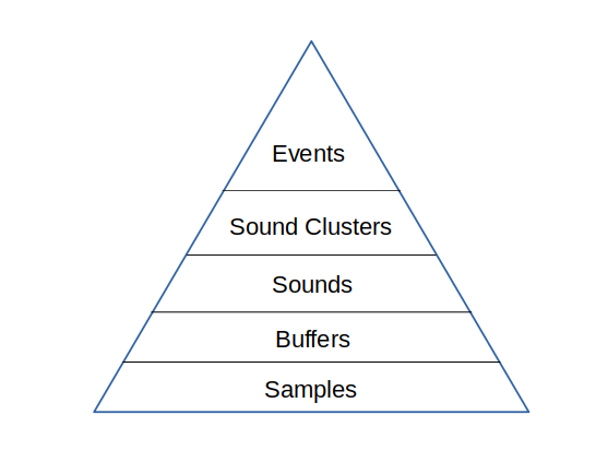
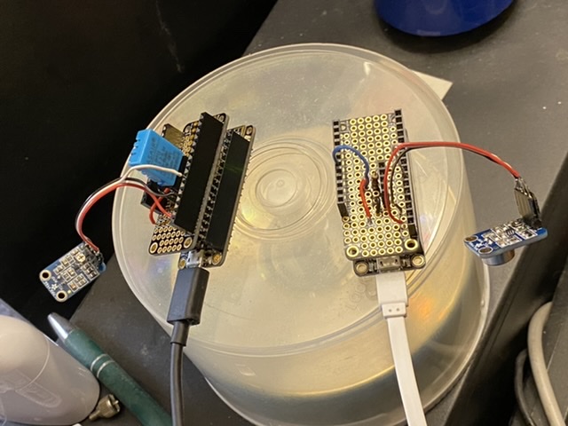
At the base of the pyramid of abstractions are samples. These are individual measurements of the voltage the microphone element produces. The samples are grouped together into buffers. Currently the size of a buffer is 512 samples, collected at approximately 20kHz. The microcontroller decides if the buffer is interesting by looking for samples where the voltage falls above a threshold. If interesting, it then forwards that buffer and preceding and following buffers to the server.

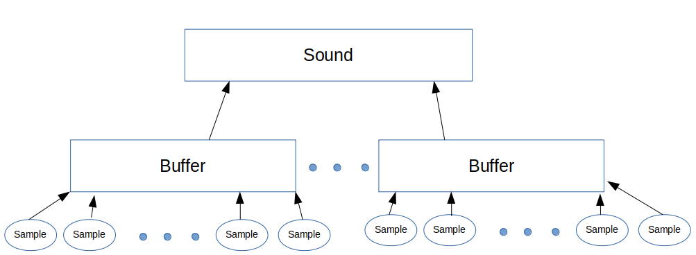
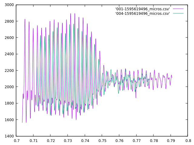
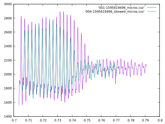
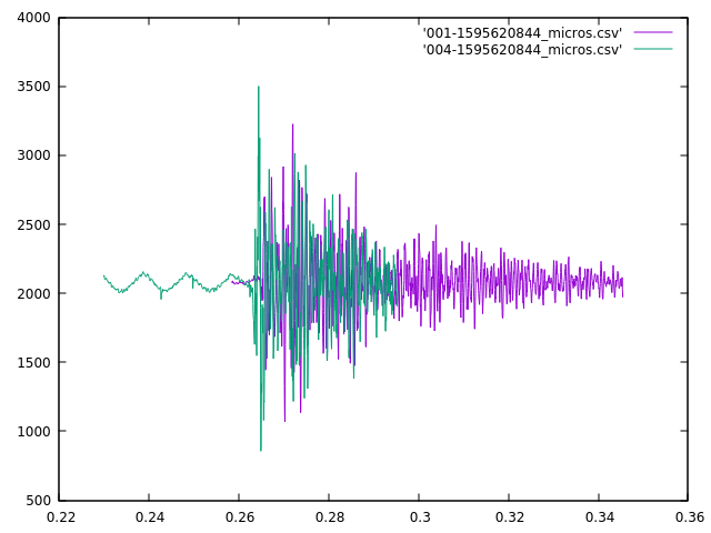
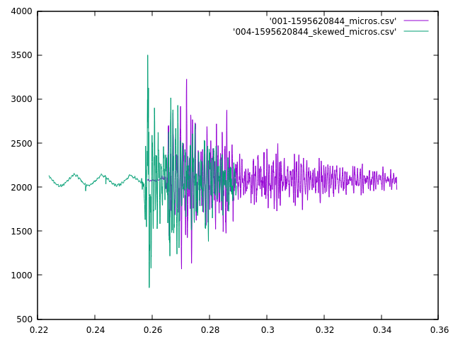
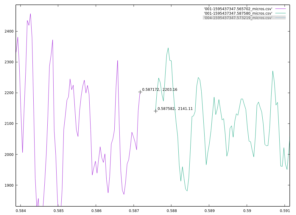
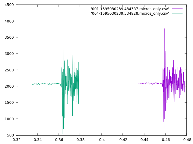
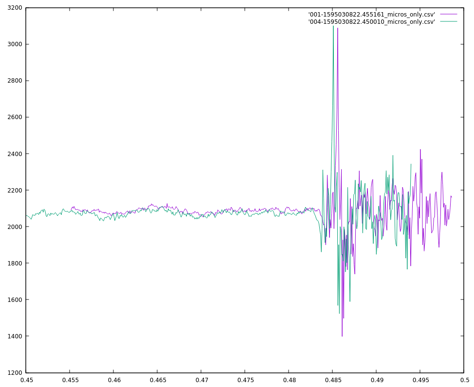
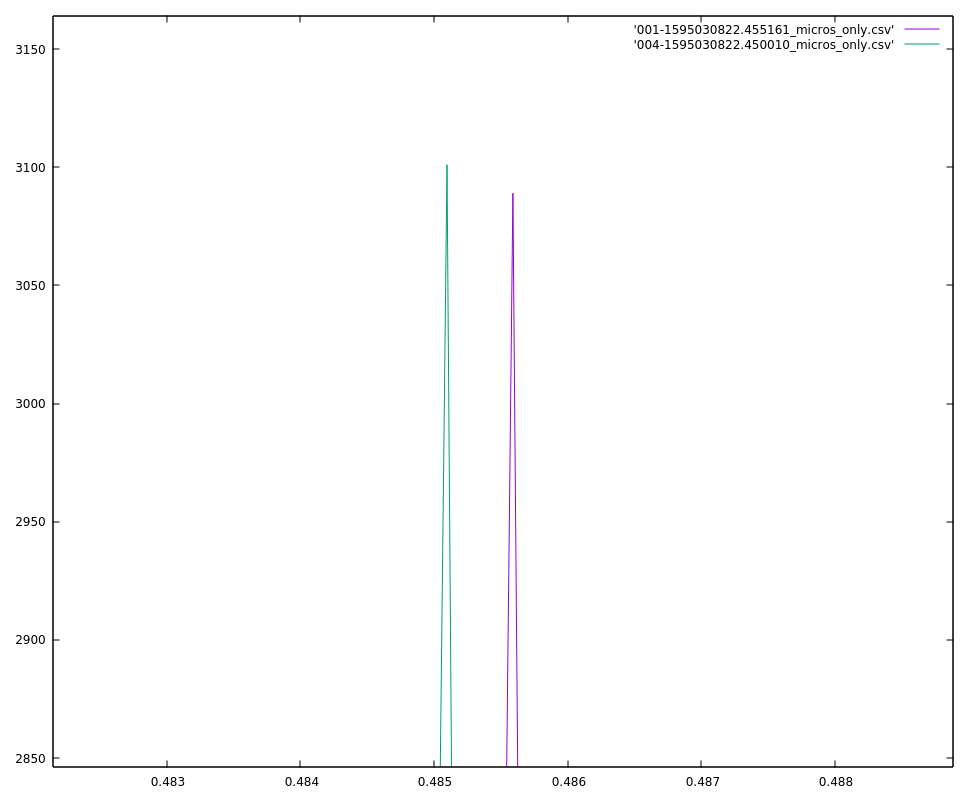
The server receives these sound buffers from an individual microphone controller. The server groups these buffers together based on time. Each buffer spans about 22 milliseconds, and buffers from the same controller that arrive within 50 ms of each other are considered to be part of the same sound (50 ms chosen so that 1 or 2 dropped buffers don’t break up a single sound.)

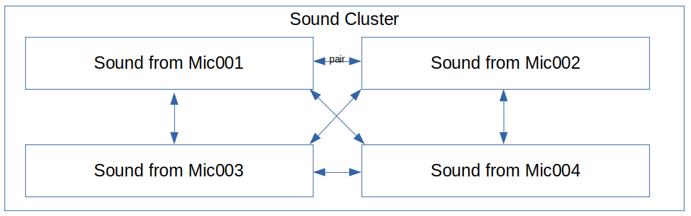
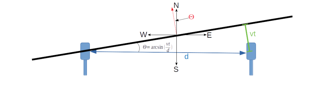
Sounds from different microphone controllers are grouped together by the server into sound clusters that occur within some small time frame that will be bounded by the time it takes for sound to travel between microphones (plus some small amount to allow for timing errors.) If the sound cluster contains sounds from more than 2 microphones, it will be considered to have originated from the same event.

The server then tries to determine where the event happened. It does this by calculating the time-offsets and similarities of each pair of sounds in a cluster. If the similarity of a pair of sounds falls below some threshold then the time-offset for that pair will be discarded. The remaining time-offsets for a cluster will then be combined the the physical arrangement of their corresponding microphone assemblies and used to calculate a best-guess for the location of the event.

Only the good skew young

Maybe I was too hasty in thinking that my curve matching algorithm wasn’t going to be useful. I had a few loud booms go off tonight with 4 mics scattered around the office and the windows open. Mics 1 and 4 were by the open window, and mics 2 and 3 were by my computer about 6 ft. (1.8 m) away. All 4 detected at least one of the big echoing booms. My algorithm gave reasonable offsets and reasonable waveform matches once skewed.

Mic 2 skewed back by 5.06 ms.

All 4 skews were in the 5 to 7 ms range, which is right about what I’d expect for microphones that were 6ft. apart on the direction of travel (6ft/1127fps = 0.005324 seconds, or 5.3 ms). Now to be fair, this was pretty much a best-case scenario for my algorithm. These were long, low rumbling booms rather than simply a loud crack. Still.. Mics 1 and 4 heard the crack at the beginning and mics 2 and 3 didn’t, and it didn’t throw off the algorithm.

To skew or not to skew

After writing up my (computationally intensive) code to measure the skew between the signals from two microphones, I’ve made a discovery. It works great for stuff with complex, low-frequency sounds like my chair creaking, but not so well in other cases. For sustained, constant frequency sounds (like beeps) it gets confused about which of several possible alignments are “best”. Take for example this short beep as heard by two adjacent microphones:

My visual best fit says the green waveform needs to be shifted a few hundred microseconds to the right, and that these were almost in alignment already. However, my algorithm shifted it ~13,000 microseconds to the left.

It did make the wave peaks line up, but since this is a more or less steady tone, that happens every couple of milliseconds. I’m also sure it maximized my fit function, but to my eye the overall envelopes don’t match nearly as well. I think there are two factors working against my algorithm here. First, the waveforms weren’t complete–the beginning of the waveforms was cut off by different amounts in the different samples. I’ve taken measures to reduce the likelihood of that happening, but I can’t eliminate it altogether. Second, this was a fairly steady tone–as I already mentioned, and there were lots of “pretty good” fits that it had to choose from.

The other situation that it doesn’t handle well is more problematic. It appears that for short, sharp sounds–like a clap, whip crack, fireworks or gunshots–there is too much high-frequency information that the two mics will sample differently, and since my sampling rate is about 20kHz, I really can only differentiate frequencies below about 10kHz (5kHz for a good fit). See the Nyquist-Shannon theorem for a more complete discussion as to why. So, when I have a signal with a lot of high-frequency information, I can’t really match it effectively. Take this example of a clap when the mics where a few feet apart (1-2 meters):

The apparent shift shouldn’t need to be large, but the algorithm doesn’t pay attention to that, and it came up with a fit that looked like:

This is a much worse fit according to my eye. I think a better technique in this case it to line up the beginning of the loud sounds, but I need to come up with a way to identify those algorithmically. I’ll probably use some heuristic like looking at the time of the first samples to fall significantly further from the mean than I’d been seeing previously, but that requires that I have a nice quiet section before the sound happens. I’ve taken steps to try to make sure that I have that (by sending the prior buffer as well when I detect an anomaly), but it doesn’t always work out as you can see in the purple curve.

The good, the bad, and the skewed

One of the technical challenges in this project is to figure out the exact time offset of two waveforms. I think I’ve solved that sufficiently.

The Good

My algorithm correctly detects the time skew of two waveforms. Here’s the raw data from two mics:

Without correction, the two waveforms look disjoint

And here’s after the skew is corrected for:

With the curve from Mic 004 skewed forward by 2.44 milliseconds

The two waveforms are a very good match.

The Bad

The algorithm is very computationally intensive. My first pass at the code, finding the skew took 10-20 minutes for two 50 millisecond waveforms. With a little optimization from caching interpolation results and discarding excess precision, I got it down to 1-2 minutes (much better, but still pretty slow. I may be able to get another factor of 2 or 3 my switching to C++ from Python, but getting the code right will be more difficult.

The Skewed

It has occasionally detected skews in the range I’d expect for two microphones next to each other (a few hundred microseconds), but most of the skews have been in the 2-2.5 millisecond range, which is about 10 times what I’m hoping for. More work on time sync is needed apparently.

Mind the gap

The downside to increasing the sample rate is that I also increased the timing error that accumulates during a sampling buffer. Look at these sequential data buffers:

I’ve got a gap

There’s a gap of more than 400 microseconds between the last measurement of the first packet and the first measuement of the second. That gap isn’t real though. There’s actually about a 42-43 microsecond gap in real time, but because I send the measurement interval as a whole number of microseconds between messages, there’s a fraction of a microsecond that gets lost to truncation. In this case, the actual interval of 42.72 microseconds gets truncated to 42 microseconds when sent to the server, and that means that there’s about a 370 microsecond error by the end of the packet (0.72 microseconds * 512 measurements in the packet).

Currently the measurement packet has a 22 bytes of header, including both the timestamp of the beginning of the packet (8 bytes) and the number of microseconds between measurements (2 bytes). I could redesign the measurement packet so that the same two bytes pass 100ths of microseconds rather than whole microseconds, and that would allow up to 655.35 microseconds as a measurement interval without changing the overhead of the packet. (I’ve only got about 1450 bytes to work with in a UDP packet that’s going to travel over WiFi and Ethernet, so I’m trying to be frugal with headers and leave as much space as possible for actual measurements.)

Crank up the frequency

I have been assuming that approximately 10kHz was about the maximum sampling rate I could achieve, but it turns out I was very wrong. So far I’ve gotten up to approximately 20kHz and am not seeing any degradation in performance. I’m not sure how high I can (or should) crank this up for optimal system performance, but I’ve already increased the precision from 1 reading every 85 microseconds to 1 every 42 microseconds. Now if only my clock were that accurate.

And now for the time and temperature…

I’ve been noticing that the microphone that has the DHT-11 temperature sensor consistently under-performs the other microphone in terms of how well is stays in sync with the NTP server. I have documented previously that trying to read a non-existent sensor caused major sync issues, but I now know that even if the sensor is working properly, it still throws the sync off slightly.

On mic 001 (the one with the temperature sensor). I was seeing the average offset being somewhere around +/-1300 microseconds, whereas on mic 004 (the one without the sensor or code to read it). I was typically seeing offsets of +/-300-400 microseconds (1/4 to 1/3 as large). So I disabled the DHT-11 on mic 001, and within 15 minutes the average offset was +/- 400-500 microseconds, and the timing of received sound waves was much more in sync.

I have no idea what this was, but both mics agree when it was.

And zooming in on that first big positive peak you can see that they’re only about 400 microseconds apart, which is pretty good.

.9093730-.909344 = .000386 seconds, or 386 microseconds difference

It’s not the 100 to 200 microsecond offset I’m looking for, but I can live with this level of error.

Now what am I going to do with the temperature sensor? I still need to be able to measure ambient air temperature to calculate the speed of sound accurately, but it was never a requirement that I have 4 of them or that they be co-located with microphones. I have some spare ESP8266 feathers now, and while they’re not good for the microphones, I can easily re-purpose them to being a couple of temperature sensors. I’ll play with low-power deep-sleep and have them wake up every 30 seconds or so to check the temp and report in. That should give me a fairly accurate and current air temp.

ESP32 not working out

Since the ESP8266 wasn’t working for this project, I ordered a Feather Huzzah ESP32, which features a slightly newer Wifi chip from Espressif. I had high hopes that this would be a cheaper alternative to the M0 feather, since it had a math-coprocessor and dual cores. I thought the second core could handle the 10kHz interrupt routine to read the microphone while the primary core did all the I/O with the WiFi.

It seemed to work well initially, but the processors starting panicking and resetting every few seconds. I built a test rig, and it was able to handle reading the mic at 10kHz no problem, however, as soon as I added my NTP routines to timestamp the buffers, then it reset almost immediately. My first thought was that the NTP estimation routine was slow enough to cause the interrupt service routine (ISR) to bleed into the next firing of the timer interrupt, but after a little research there appears to be another problem.

When I ripped out the hairy math that did time skew estimation and replaced it with slightly less hairy math, I used floating point calculations. I thought that the ESP32, with it’s dedicated floating-point co-processor would make quick work of these, and it probably does, but doing floating point math in the ISR is apparently a no-no. Maybe because the coprocessor uses interrupts to signal that it has completed its calculation, and that having interrupts within interrupts was causing a race condition of some kind, and that was occasionally reseting the chip.

So now I either have to go back to hairy integer math in the skew estimation routine, or I need to stick to the M0. I think I’ll stick with the M0, and swallow the additional $15 per microphone.

Another timing bug squashed

I spent several hours trying to figure out why my circuit on the second M0 microcontroller was having significant timing issues when the first M0 wasn’t. The second M0 didn’t seem to exhibit the problem in my NTP test rig either. I finally figured it out. As you can see below, when I built the second M0, I didn’t have a second DHT-11 temperature and humidity sensor (the blue box–I forgot to order a second one), but I kept the code the same. If I use the preprocessor flag I put in my code to disable all the DHT related calls, the timing issues go away.

Two microphones listening for booms

Here’s my theory as to what’s happening. The DHT11 product page on Adafruit’s site says that reading the chip requires careful timing. To get the timing right, I suspect that it disables interrupts while reading the chip. If the chip is there then this only takes a few microseconds, and nobody is the wiser. However, if the chip isn’t there, it has to wait for some timeout to happen, and that means interrupts are disabled for a while, and that throws off the millis() and micros() timing functions, which won’t increment while interrupts are disabled. Since my NTP library uses micros() calls frequently to calculate the time since the last server sync, it was accumulating significant errors which were causing the readings to go all over the place.

By the time I’d figured this out, I’d already ripped out a lot of the hairy math I had implemented for calculating gradual skews and correction factors, and replaced it with slightly less hairy math. It’s far more straightforward and easy to understand, and the only downside is that a lot of it is now floating point math, which is slower on some microprocessors.

I’m still seeing about a 1-2 millisecond skew between the readings on the two microphones, and I’m going to have to find a way to adjust for that.

Okay results with 2 microphones

I fixed the previously mentioned time jump problem, at least well enough.

I also now have 2 (roughly) identical microphones set up, and while the initial results were frightening, they settled in and starting behaving reasonably.

My first attempt was right after I had plugged them both in, and the result was this:

Initial skew from M0 microphones
Nowhere close

There was about 90-100 millisecond skew in their readings, which since they were right next to each other, seemed very odd. It’s the kind of delta I would expect if they were 50 meters (165 ft) apart. I thought that maybe my time sync wasn’t nearly as stable as I thought it was, but I decided to give them some time to settle-in and converge, and that helped. After 10 seconds of being on, I got this result:

Microphone skew after settling in
almost synced

This was much more encouraging. The waveforms are almost synced. If I zoom in on the peaks, I can see a better estimate of their delta:

Zoomed in on skew after settling
Looking much better zoomed in.

The actual time difference was about 400-500 microseconds, and at least part of that (maybe 100-200 microseconds) might be due to them being 6 inches apart. This is much closer to the kind of synchronization I’m going to need for this project.

Update: Celebration premature it turns out. I still have serious NTP sync issues that are causing the two microphones to fall out of sync. Ripped out my previous hairy math and trying to fix it now, but still having problems with the corrections oscillating wildly.